Integrating scCAT-seq cell lines
Imports
[ ]:
# Biology
import muon as mu
import scanpy as sc

import mowgli
[2]:
# Plotting
import matplotlib.pyplot as plt
import seaborn as sns
Load data
Load the Liu cell lines dataset, which contains 3 well separated cell lines profiled with scRNA-seq and scATAC-seq. You can download the data from https://figshare.com/s/fadcb181b470d32c73c7
[ ]:
mdata = mu.read_h5mu("liu_preprocessed.h5mu.gz")
For computational reasons, in this simple demonstration we reduce the number of features a lot.
[4]:
sc.pp.highly_variable_genes(mdata["rna"], n_top_genes=500)
sc.pp.highly_variable_genes(mdata["atac"], n_top_genes=500)
Visualize independant modalities
Let us visualize the cell lines independantly using UMAP projections.
[5]:
# Umap RNA
sc.pp.scale(mdata["rna"], zero_center=False)
sc.tl.pca(mdata["rna"], svd_solver="arpack")
sc.pp.neighbors(mdata["rna"], n_neighbors=10, n_pcs=10)
sc.tl.umap(mdata["rna"], spread=1.5, min_dist=0.5)
[6]:
# Umap ATAC
sc.pp.scale(mdata["atac"], zero_center=False)
sc.tl.pca(mdata["atac"], svd_solver="arpack")
sc.pp.neighbors(mdata["atac"], n_neighbors=10, n_pcs=10)
sc.tl.umap(mdata["atac"], spread=1.5, min_dist=0.5)
[7]:
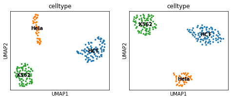
# Display UMAP
fig, axes = plt.subplots(1, 2, figsize=(8, 3))
sc.pl.umap(
    mdata["rna"],
    color="celltype",
    legend_loc="on data",
    size=50,
    show=False,
    ax=axes[0],
)
sc.pl.umap(
    mdata["atac"],
    color="celltype",
    legend_loc="on data",
    size=50,
    show=False,
    ax=axes[1],
)
plt.show()
Train model
Let us define the model and perform the dimensionaly reduction.
[8]:
# Define the model
model = mowgli.models.MowgliModel(latent_dim=5)
[9]:
# Perform the training.
model.train(mdata)
4%|▍ | 8/200 [00:08<03:32, 1.11s/it, loss=-0.11106829, mass_transported=0.757, loss_inner=-0.053246647, inner_steps=60, gpu_memory_allocated=0]
Visualize the embedding
Now, let us display the obtained embedding.
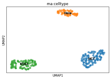
[10]:
# First using a UMAP plot. This is pure Scanpy!
sc.pp.neighbors(mdata, use_rep="W_OT", key_added="mowgli")
sc.tl.umap(mdata, min_dist=0.5, spread=1.5, neighbors_key="mowgli")
sc.pl.umap(mdata, color="rna:celltype", size=200, alpha=0.7, legend_loc="on data")
[11]:
# Then using a dendogram.
mowgli.pl.clustermap(
    mdata,
    obsm="W_OT",
    yticklabels=False,
    figsize=(5, 5),
    col_cluster=False,
)
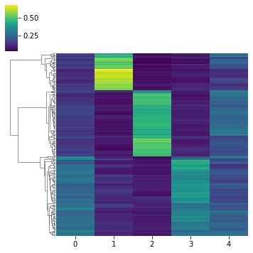
[12]:
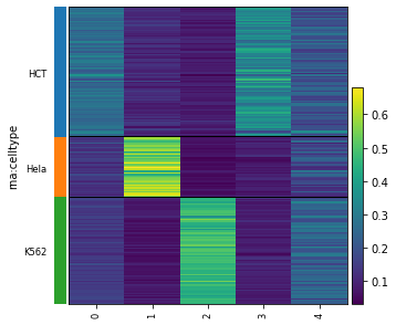
# Then, using a heatmap.
mowgli.pl.heatmap(
    mdata,
    obsm="W_OT",
    groupby="rna:celltype",
    figsize=(5, 5),
)
/users/csb/huizing/anaconda3/lib/python3.8/site-packages/scanpy/plotting/_anndata.py:2414: FutureWarning: iteritems is deprecated and will be removed in a future version. Use .items instead.
  obs_tidy.index.value_counts(sort=False).iteritems()
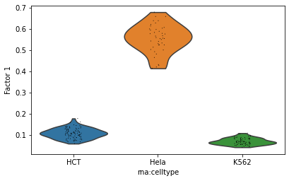
[13]:
# Finally, display a violin plot of the value at a given dimension of the cells.
mowgli.pl.factor_violin(mdata, groupby="rna:celltype", dim=1)
Clustering
We can perform clustering on the lower-dimensional space.
[14]:
# Again, pure Scanpy for clustering.
sc.tl.leiden(mdata, resolution=0.1, neighbors_key="mowgli")
[15]:
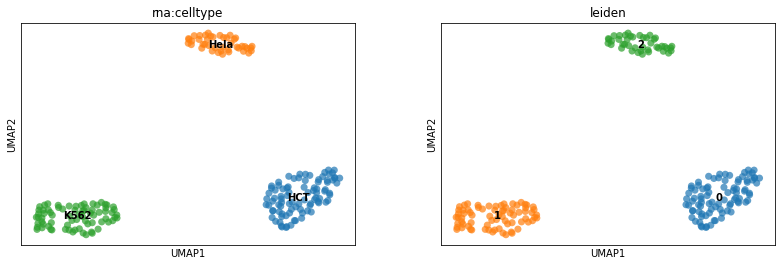
# Let's display the clustering results on the previously computed UMAP.
sc.pl.umap(
    mdata, color=["rna:celltype", "leiden"], size=200, alpha=0.7, legend_loc="on data"
)